In a previous post we considered averaging quantities built from tensors over all angles. We know wish to extend the ideas in that post to integrals of the form
\[\langle e^{\bf n^T H n} \rangle = \int e^{H_{ij} n_i n_j} \frac{d\Omega^d_{\bf n}}{S_d} = f_d({\bf H})\]where \(H_{ij}\) is a second rank tensor, symmetric without loss of generality. Ideally, we would like to reason what the solution looks like in arbitrary dimension.
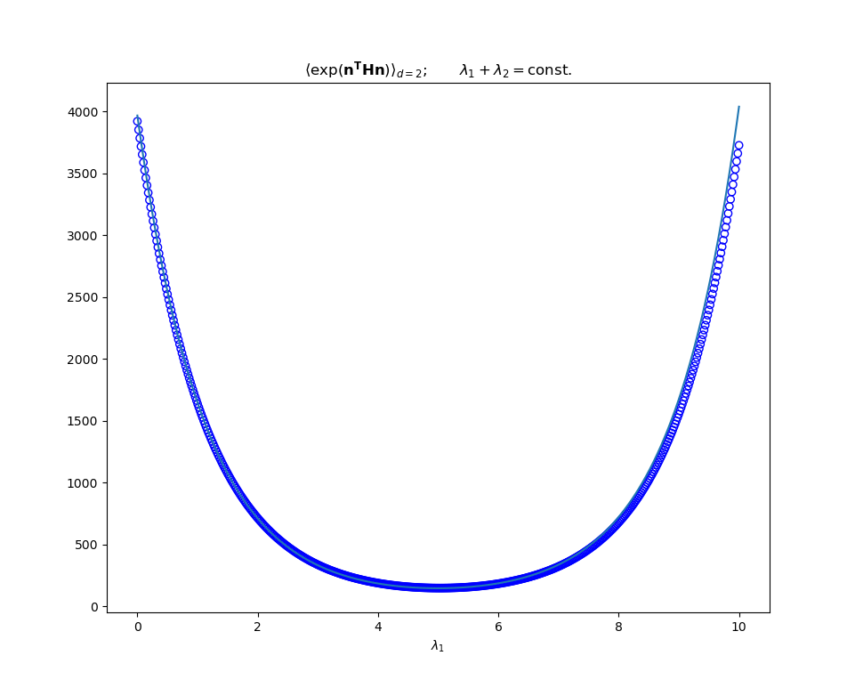
Specific solutions can sometimes be worked out directly. For exmaple in \(d = 2\) we can diagonalise the quadratic form in the exponent (it is a scalar and invariant to the choice of basis, and the integration measure doesn’t change under a rotation of the axes)
\[\begin{equation} \label{eq:f2} \tag{1} f_2({\bf H}) = \int e^{\lambda_{1} \cos^2 \theta + \lambda_2 \sin^2 \theta} \frac{d\theta}{2\pi} = e^{(\lambda_{1} + \lambda_{2})/2} I_{0}\Big(\frac{\lambda_{1} - \lambda_{2}}{2}\Big) \end{equation}\]where \(\lambda_{1, 2}\) are the eigenvalues (i.e the invariants) of \(\bf H\). As expected, the result is symmetric under the exchange of eigenvalues. How else might we derive Eq \ref{eq:f2}?
\(d\)-dim
The first thing to notice is that we can decompose a symmetric rank two tensor into a isotropic part and a symmetric traceless part i.e \(H_{ij} = \frac{H_{kk}}{d} \delta_{ij} + T_{ij}\). Which simplifies our expression to
\[f_{d}({\bf H}) = e^{H_{kk}/d} \int e^{T_{ij} n_{i} n_{j}} \frac{d\Omega^d_{\bf n}}{S_{d}} = e^{H_{kk}/d} f_{d}({\bf T})\]Assuming \(\bf T\) is normal, the next thing to do is diagonalise the quadratic form to yield
\[f_{d}({\bf T}) = \int e^{ \sum_{i\neq j}^d \lambda_i (n_i^2 - n_j^2)} \frac{d\Omega^d_{\bf n}}{S_{d}}\]Where again \(\lambda_i\) denote the eigenvalues of \(\bf T\) (and thus \(\bf H\), up to a linear transformation). The appearance of the peculiar \(-n_j^2\) is to enforce the traceless-ness of \(\bf T\). Note that we can easily see that (\(\partial_k \equiv \partial_{\lambda_k}\))
\[\sum_{k=1}^{d-1} \partial_{k} f_{d} = f_{d} - (d+1) \int n_j^2 e^{ \sum_{i\neq j}^d \lambda_i (n_i^2 - n_j^2)} \frac{d\Omega^d_{\bf n}}{S_{d}} \label{eq:plane-pde} \tag{2}\]The result should clearly be independent of \(j\). Already it looks like diagonalising too soon has led us down an annoying path.
Let us return to the non diagonlised expression for \(f_d({\bf T})\). Due to \({\bf n}\) being of unit magnitude, we derive 2 expressions:
\[\begin{equation} \frac{\partial}{\partial T_{km}} \frac{\partial f_{d}({\bf T})}{\partial T_{km}} \equiv \frac{\partial }{\partial {\bf T}} : \frac{\partial f_{d}({\bf T})}{\partial {\bf T}} = f_d({\bf T}) \end{equation}\] \[\begin{equation} \frac{\partial f_{d}({\bf T})}{\partial T_{kk}} = f_d({\bf T}) \end{equation}\]A first order and second order equation. The first order equation is merely telling us that \(f_d\) has a factor like \(e^{T_{kk}/d} = 1\), so isn’t so interesting. Indeed, this was similar to the contribution we separated out from the begining when decomposing our original \({\bf H}\). The second order one has more structure to unpack. If we consider this in the principal frame then we get another differential equation governing \(f_d\)
\[\sum_{i\neq j}^d \partial_i^2 f_d = f_d\]And so we get some of the laplacian again. Not that unlike the case in the previous post, where we took a derivative in a vector’s components, here the inteesting invariant is not the sum square of the components of the Laplacian. The exception is 2-dim, where \(\lambda_1 = -\lambda_2 \equiv \lambda\) and so \(\sqrt{\lambda_1^2 + \lambda_2^2} = 2^{1/2} \lambda\), so the “radial” variable contains all the information you would need. This explains how \(I_0(\lambda)\) arose in the explicit calculation above in 2-dim; it is the solution to the 2-dim radial Helmholtz equation.
For \(d>2\) the correct variables to use are not as straight forward to deduce. The typical coordinate systems you could define in d-dim (cartesian, radial etc) are not the most natural choice, but could be used in the standard separation of variables way to yield a series solution. In that sens the problem is solved - you just need to apply the boundary conditions afterword.
From here it seems hard to proceed. We can say some basic things, such as that \(f_d\) is obviously bounded by the range of eigenvalues
\[e^{\lambda_{\rm max}} \geq f_d \geq e^{\lambda_{\rm min}}\]And can be represented as a multivariable taylor series
\[f_d = \sum_{k_1 k_2 ... k_d}^{\infty} \frac{\langle n_1^{2 k_1} n_2^{2k_2} ... n_d^{2k_d} \rangle}{k_1! k_2! ... k_d!} \lambda_1^{k_1} \lambda_2^{k_2}...\lambda_d^{k_d}\]Not much insight (yet).