Oftentimes we must do some form of average to calculate an expected quantity. In this post we’ll consider doing angular averages of scalar functions of vectors in various dimensions. We’ll first consider integrals of the form
\[\langle f( {\bf{a_1}}, {\bf{ a_2}}, .., {\bf{ n}}) \rangle = \int f( {\bf{a_1}}, {\bf{ a_2}}, .., {\bf{ n}}) \frac{d \Omega_n}{2 \pi}\]where the integration domain is over all directions the unit vector \(\bf{n}\) can take. These integrals can occur during perturbative calculations for non-equilibrium field theories, for example. Let’s first consider a subset of expressions - \(f_{\Pi_n} = (\bf{a_1} \cdot \bf{n}) (\bf{a_2} \cdot \bf{n})...(\bf{a_n} \cdot \bf{n})\). How might we perform such an average? Note that using the summation convention we can write this expression as
\[\langle f_{\Pi_m}({\bf a}_i) \rangle = (a_1)_{i_1} (a_2)_{i_2}...(a_m)_{i_m} \int n_{i_1} n_{i_2} ... n_{i_m} \frac{d \Omega_n}{2 \pi}\]The integrand is now a tensorial quantity. The integral should be invariant under rotations of the unit vector in the integrand as we integrate over all angles. As the integral is a tensor invariant under rotation transformations it will be isotropic, and we can therefore restrict the form to
\[\int n_{i_1} n_{i_2} ... n_{i_m} \frac{d \Omega_n}{2 \pi} = \mathcal{A}_m I_{i_1 i_2 ... i_m}\]where \(I_{i_1, i_2, ...,i_m}\) is the general isotropic tensor. It should be symmetric under the exchange of any two indices, (this means the tensor is identically 0 for an odd number of vectors, as the isotropic tensor of odd rank must involve the totally antisymmetric tensor). In even dimension we can write \(I\) as a sum of the products of kronecker delta’s, with all possible pairings.
The first 2 non-zero tensors of this type are
\[\begin{equation} \int n_i n_j \frac{d \Omega_n}{2 \pi} = \mathcal{A}_2 \delta_{ij} \\ \int n_i n_j n_k n_l \frac{d \Omega_n}{2 \pi} = \mathcal{A}_4 ( \delta_{ij} \delta_{kl} + \delta_{ik} \delta_{jl} + \delta_{il} \delta_{jk} ) \\ ... \end{equation}\]To evaluate the coefficients is fairly easy, we merely choose any easy to calculate component. For example we can choose all indices \(= 1\).
\[\begin{equation} \begin{aligned} \int n_{1} n_{1} ...n_{1} n_{1} \frac{d \Omega_n}{2 \pi} &= \mathcal{A}_{2m} \frac{(2m)!}{2^m m!} \\ &= \int ( \cos \theta)^{2m} \frac{d\theta}{2\pi} \\ \implies \mathcal{A}_{2m} = \frac{1}{2^m m!} \\ \end{aligned} \end{equation}\]Now we can evaluate \(f_{\Pi_{2m}}\).
\[\begin{equation} \begin{aligned} \langle f_{\Pi_n}({ {\bf a}_i} ) \rangle &= \int f( {\bf{a_1}}, {\bf{ a_2}}, .., {\bf{ n}}) \frac{d \Omega_n}{2 \pi} \\ &= \mathcal{A}_{2m} \times ( \text{sum of all possible dot product pairs}) \\ \end{aligned} \end{equation}\]Consider another integral
\[\begin{equation} \begin{aligned} \langle e^{\bf{ c \cdot n}} \rangle &= \int e^{\bf{c} \cdot \bf{n}} \frac{d \Omega_n}{2 \pi} \\ \end{aligned} \end{equation}\]This can also be done in a systematic way by taylor expanding the integrand \(( c = \vert {\bf c} \vert)\).
\[\begin{equation} \begin{aligned} \langle e^{\bf{ c \cdot n}} \rangle &= \sum_k \frac{1}{k!} f_{\Pi_k} \\ &= \sum_{l=0} \frac{1}{(2l)!} \frac{1}{2^{k+1}} \begin{pmatrix} k \\ k/2 \end{pmatrix} (c^2)^k \\ &= \frac{1}{2} \sum_{l = 0}^{\infty} \frac{1}{(l!)^2} (c/2) ^{2l} = I_0( c ) \\ \end{aligned} \end{equation}\]where \(I_0(x)\) is the zeroth order modified bessel function of the first kind.
But there are more general tricks we can play. Notice that since these integrals are done over solid angles, the final answer must depend on the magnitude of the vectors (and dot products between them if there is more than one unique vector involved). Let us examine \(\langle e^{\bf{ c \cdot n}} \rangle\), and this time take a vector derivative.
\[\begin{equation} \begin{aligned} \nabla_{\bf c} \langle e^{\bf{ c \cdot n}} \rangle &= \int {\bf n} e^{\bf{c} \cdot \bf{n}} \frac{d\Omega_{\bf n}}{2 \pi}\\ \nabla_{\bf c} \cdot \nabla_{\bf c} \langle e^{\bf{ c \cdot n}} \rangle &= \int n^2 e^{\bf{c} \cdot \bf{n}} \frac{d\Omega_{\bf n}}{2 \pi} = \langle e^{\bf{ c \cdot n}} \rangle \\ \end{aligned} \end{equation}\]since \(\langle e^{\bf{ c \cdot n}} \rangle\) can only depend on the magnitude of the vector \(\bf c\), \(\nabla_{\bf c} \cdot \nabla_{\bf c}\) must be the radial part of the laplacian in \(d = 2\).
\[\begin{equation} c^{-1} \partial_c \Big( c \partial_{c} \Big( \langle e^{\bf{ c \cdot n}} \rangle \Big) \Big) = \langle e^{\bf{ c \cdot n}} \rangle \end{equation}\]Solving the equation with the boundary conditions at \(c = 0, \infty\) again gives us \(I_0( c )\).
The advantage of this sort of reasoning compared to the more direct method is that it is clear how it generalises to other dimensions - just replace with the radial part of the laplacian with appropriate dimension. For example in \(d = 3\) the angular integral can be seen to be
\[\begin{equation} \langle e^{\bf{ c \cdot n}} \rangle = \frac{\sinh(c)}{c} \end{equation}\]Indeed we can work out the solutions for any \(d > 1\)
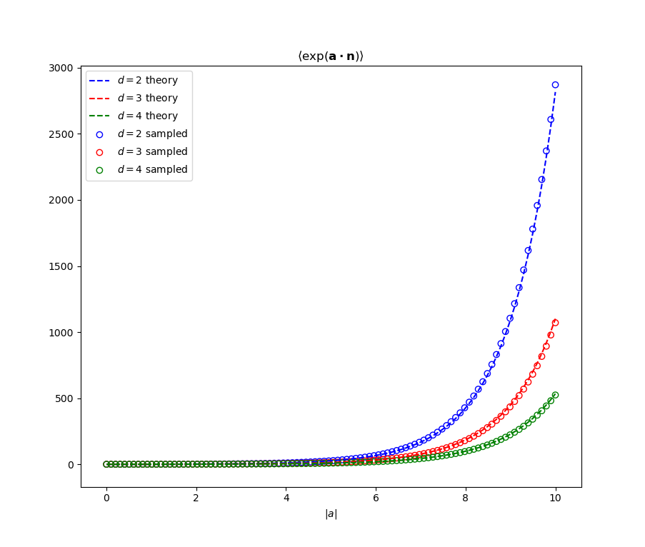
\[\begin{equation} \langle e^{\bf{ c \cdot n}} \rangle = \frac{2^{d/2 - 1} \Gamma(d/2)}{c^{d/2 - 1}} I_{d/2 - 1} (c) \end{equation}\]where \(\Gamma\) is the Gamma function. The figure below shows agreement between the analytic results and evaluation of \(\langle e^{\bf{ c \cdot n}} \rangle\) via sampling points on a sphere, for some small values of \(d\).
Higher order tensors should follow the same ideas - the averaged quantities should only depend on the (in general non-linear) invariants of the tensor. Quantities like
\[\begin{equation} \langle e^{\bf{n^T H n}} \rangle = \int e^{H_{ij} n_i n_j} \frac{d\Omega^d_{\bf n}}{S_d} \end{equation}\]will be considered in a later post (i.e when i get to it).
References:
[1] NIST Digital Library of Mathematical Functions