Arguably one of the simplest, nicest to work with distributions is that of a Gaussian. Within the field of stochastic ODEs, the common stochastic noise (the Weiner process) is simply a Guassian distributed point process. But depending on the system in question, a systems noise could be distributed differently. Some of these cases are of interest, as they can describe the breaking of fluctaution dissipation and memory effects in stochastic systems. The point here is that if the system is linear then the problem is no harder if we can represent the noise as some linear combination of gaussian point processes.
Let us consider the most basic example. Consider the single variable stochastic system
\[dx_t = \lambda + \mu x_t dt + d \Pi_t\]\(d \Pi\) is a stationary stochastic noise, but can be a peculiar one. It isn;t distributed according to a gaussian, but instead it follows some general symmetric distribution \(\mathcal{P}(d \Pi_t = x) = \rho(x)\). What we want to be able to do is find some continuous superposition of functions of zero mean gaussians which mimic \(\rho\). i.e
\[\int_{0}^{\infty} f_L(\beta) e^{- \beta x^2 /2}\frac{d\beta}{\sqrt{2 \pi \beta^{-1}}} = \rho(x) \label{eqn:integral_f} \tag{1}\]We also want to derive conditions for when this is even possible. But first let’s do a quick example to be clear.
Example: Lorentzian Distribution
Suppose we wanted to represent a Lorentzian distribution in this manner. The Lorentzian pdf is well known and corresponds to a Cauchy Process, which is a discontinuous jump process.
\[\int_{0}^{\infty} f_L(\beta) e^{- \beta x^2 /2}\frac{d\beta}{\sqrt{2 \pi \beta^{-1}}} = \frac{1}{\pi} \frac{\delta}{x^2 + \delta^2}\]After a few redefinitions we can write the same expression as
\[\int_{0}^{\infty} F_{L}(\beta') e^{- \beta' s} d\beta ' = \frac{1}{\pi} \frac{\delta}{s + \delta^2}\]We can spot the answer from here, either by inspection or noticing that this Laplace Transform is well known and it’s inversion can be looked up in a table. This then gives that
\[F_L(\beta') = \frac{\delta}{\pi} e^{-\delta^2 \beta'}\]which then leads to
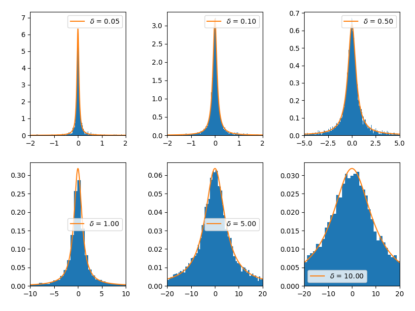
\[f_L(\beta) = \frac {\delta }{\sqrt{2 \pi}} \beta^{-1/2} e^{-\delta^2 \beta/ 2} = \Gamma(1/2, \delta/\sqrt{2})\]This is Gamma distributed. It follows that we can calculate observables for a gaussian process with noise \(\sqrt{2/\beta} dW_t\) and then perform a secondary average over \(f_L(\beta)\) (as long as the system is linear) to get the observables in the Cauchy process. From a simulation perspective, we can get the same behaviour by, at every timestep, randomly choosing \(\beta\) according to \(f_L(\beta)\). One way to think about it is having a system coupled to many different equilibrium heat baths with various strengths, which then gives rise to seemingly nonequilibrium noise behaviour. Below is a picture showing that we do indeed get a good mimic
With \(f_L\) positive we could view it as a sort of meta ensemble of variances, or a Superstatistical ensemble to use a term coined by E Cohen. We could then simulate the process by seeing it as some kind of frequency for each variance over the simulation. Table 1 shows a table showing how to get define \(f(\beta)\) in order to get certain target distributions. It shows that we can get some quite varied staitistical features, such as broad tails or exponential decay.
\[\begin{array}{c|lcr} \text{Behaviour} & \rho(x) & f(\beta) \\ \hline \text{Laplace distribution} & c \exp(-c \vert x \vert )/2 & \propto \exp(-c^2/2 \beta)/c \beta^2 \\ \text{t-distribution} & \propto (1 + x^2/\nu)^{-(\nu + 1)/2} \sim \vert x \vert ^ {-\nu - 1} & \propto \beta^{\nu/2 -1} \exp(-\beta \nu/2) \\ \text{Lorentzian} & \delta (x^2 + \delta^2)^{-1}/\pi & \Gamma(1/2, \delta/\sqrt{2}) \\ \end{array}\]We can do better than just resorting to a lookup table or inspiration if we wish to get a certain target distribution. We can systematically construct a differential equation for \(f\) given the target (if such an \(f\) exists). for example suppose now we wish to create the Exponential distribution
\[\int_{0}^{\infty} f_E(\beta) e^{- \beta x^2 /2}\frac{d\beta}{\sqrt{2 \pi \beta^{-1}}} = \frac{c \exp(- c \vert x \vert) }{2}\]We know that for \(x>0\) the RHS obeys the ODE \(y'' - c^2y = 0\) (we only need to constrain half the distribution, as we automatically get something symmetric from the gaussian mixture construction). Therefore let us take a double \(x\) derivative on both sides of the equation
\[\int_{0}^{\infty} F_E(\beta) \big( - \beta + (- \beta x)^2 \big) e^{- \beta x^2 /2}d\beta = c^2 \int_{0}^{\infty} F_E(\beta) e^{- \beta x^2 /2} d\beta\]After intgerating the second term on the LHS by parts we then arrive at the expression
\[\int_{0}^{\infty} \Big( (\beta + c^2) F_E(\beta) - 2 \partial_{\beta}(\beta^2 F_E) \Big)e^{- \beta x^2 /2} d\beta = 0\]This should be true for all \(x\) so the integrand identically vanishes. This differential equation can be easily solved to give
\[F_E(\beta) \propto \beta^{-3/2} \exp(-c^2/2\beta) \implies f_E \propto \beta^{-2} \exp(-c^2/2 \beta)\]Purely positive \(f\) has some limitations - it’s clear that it could not mimic distributions with a local minimum at the origin, for example. There are even stronger limits. A basic fact to consider here is that the Laplace transform of a positive integrable function is always log-concave. If \(g\) is such a function then directly from Holder’s Inequality \((1/p = \lambda, 1/q = 1 - \lambda)\) we get
\[\int_0^{\infty} g(t) e^{-[\lambda s_1 + (1 - \lambda) s_2] t } dt \leq \Bigg( \int_0^{\infty} g(t) e^{-s_1 t}dt \Bigg)^{\lambda} \Bigg( \int_0^{\infty} g(t) e^{-s_2 t} dt \Bigg)^{1 - \lambda}\]The natural next step would be to allow \(f\) to go negative at some points to mimic some \(\rho\) in the integral sense ( Eq \eqref{eqn:integral-f} ). But the RHS must always be positive. Two zero mean gaussians with \(\sigma_1\) and \(\sigma_2\) always have crossover points (Normalised gaussians do not envelope each other) so their difference will be negative in some region of space. This consideration shows us we need to have some restrictions on \(f\) if we allow it negative.
What’s more, letting \(f\) be negative is still not sufficient to describe all functions of interest. As another example consider a symmetric bimodal distribution
\[\int_{0}^{\infty} f_{BM}(\beta) e^{- \beta x^2 /2}\frac{d\beta}{\sqrt{2 \pi \beta^{-1}}} = \frac{1}{2 \sqrt{2 \pi \eta^{-1}}}\Big( e^{-\eta(x+\Delta)^2/2 } + e^{-\eta(x-\Delta)^2/2} \Big)\]For this case, we’ll fourier transform both sides in \(x\). This then yield
\[\int_{0}^{\infty} f_{BM}(\beta) e^{- \beta^{-1} k^2 /2} d\beta= e^{- \eta^{-1} k^2 /2} \cos (k \Delta)\] \[\int_0^{\infty} F_{BM}(\beta') e^{-\beta' s} d\beta' = \cos(\Delta \sqrt{s})\]More rearranging/shifting in the second line. But this equality can never be satisfied. If we look at the limit \(s \rightarrow \infty\) then the LHS should go to 0 whereas the RHS has no defined limit.
References:
[1] Crispin Gardner, Handbook of Stochastic Methods
[2] C Beck, E G D Cohen, Superstatististics