Premise
I recently came across a paper which investigates rheological properties of a material using a stochastic Levy flight process. To construct this mean field theory, it first starts by considering discretised space, with each cell/block/site \(i\) taking some local stress value \(\sigma_i\). As the elastic system undergoes relaxation, or local changes of arrangement this stress field over space will vary. These sites all interact - if one site undergoes a massive change in stress then it will effect the stress felt in other sites in a local manner.
Model
One route to modelling how the relaxation of one site \(i\) affects the stress field at site \(j\) is through the Eshelby kernel :
\[\sigma_j = \mathcal{G}_{ij}( r_i - r_j ) \sigma_i \tag{1} \label{eqn:eshelby}\]This form is well motivated from the theory of linear elasticity. The stress field at different points should be related via a propagator (Green’s function), and although there is no reason to expect amorphous solids should follow these rules in full generality, this form works quite well for them too.
This propogator takes different forms depending on the dimension \(d\) and goes like \(\sim 1/r_{ij}^d\). Now imagine a more dynamic situation, where site stresses are constantly changing, sometimes in a continutous fashion (due to something like elastic deformations) or in sharp discontinous ways (due to relaxation events). The combination of all of these changes in stress is a source of mechanical noise for the site. Although we may be tempted to use some sort of central limit argument to model this noise as Gaussian, Eq \ref{eqn:eshelby} tells us that perhaps the noise follows a different distribution. In particular, if we imagine that the small elastic deformations which change stresses at other sites to be of the same order, then the noise felt at site \(i\) should be power law, which is more broadly distributed than a Gaussian distribution. On top of this, because the sites are discretised the random mechanical noise should have some finite cut off, related to the size of each site and magnitude of average changes in stress.
So now we should write down an equation for the dynamics. A constant shear stress \(\Sigma = \sum_i \sigma_i/N\) is applied to system. Let us describe the relaxation behaviour by saying if any site’s stress \(\vert \sigma_i \vert > 1\) then it is classed as “unstable”, and after a constant time will relax to zero. Defining \(x_i \equiv 1 - \sigma_i\) we can write down how stress is redistributed in the system after a plastic event
\[x_j(l+1) - x_j(l) = \mathcal{G}_{ij}(r_i - r_j) \sigma_i(l) \tag{2} \label{eqn:model}\]The variable \(l\) is an integer numbering the number of plastic events that have occured. Now we pass over into a mean field model, where we say that each site is interacting in an identical fashion. We relax an unstable site completely, and redistribute its stress throughtout the systems \(N-1\) remaining sites evenly but with broad fluctuations on top. In this way we completely ignore any spatial information in the system.
\[x_i(l+1) = 1 \\ x_j(l + 1) - x_j(l) = - \frac{1 - x_i(l)}{N - 1} + \zeta_j\]Where \(\zeta\) is our broad noise (with zero mean). It takes values according to the distribution
\[p(\zeta) = \frac{A}{N} \vert \zeta \vert^{-1-\mu}\]with a lower cut off at \(\zeta_c = (2A/\mu)^{1/\mu} N ^{-1/\mu}\). When \(\mathcal{G} \sim 1/r^{\alpha}\) then \(\mu = d/\alpha\), so we are mostly interested in the physical case of \(\mu=1\).
We can then finally pass to a continuous description of this system by letting \(N \rightarrow \infty\) whilst keeping \(\gamma \equiv l/N\) a constant.
\[x_j(\gamma) = x_j(0) - v \gamma + \tilde \zeta_j(\gamma) \tag{3} \label{eqn:levy-flight}\]where the drift \(v\) is the mean stress of unstable sites before relaxation i.e \(v = \langle \sigma_u \rangle\) in the paper’s notation. If \(\Sigma > 0\) then clearly \(v > 0\) as well. The noise term is now an accumulation of \(\gamma N\) random kicks and we call it’s distribution (which is convolutional) \(p_{\gamma}(\zeta)\). Using a standard sort of Markovian argument we can then derive a Fokker Plank master equation for the dynamics.
\[\frac{\partial P}{\partial \gamma} = v \frac{\partial P}{\partial x} + \int^{\infty}_{\infty} [ P(y) - P(x)] w'(y - x) dy + \delta(x-1) \\ \text{with} \\ w'(x) = \lim_{\gamma \rightarrow 0} \frac{w_{\gamma}(x)}{\gamma}\]Lin and Wyart then analyse the Fokker Plank equation for various \(\mu\), looking for stationary solutions of the form \(P(x) \sim P_0 + C_0 x^{n}\) for \(x \ll 1\). From this they can deduce the psedogap exponent.
Main Results
The main results of the paper are as follows:
- for \(\mu = 1\) (the most physically relevant case, and corresponds to Levy flights) the pseudogap exponent \(\theta\) for critically sheared systems is not universal, and depends on the sytem specifics.
- There is a violation of the marginal stability hypothesis
- \(\theta\) varies non-monotonically with stress, a result which was previously unexplained (even qualitatively)
Other Considerations
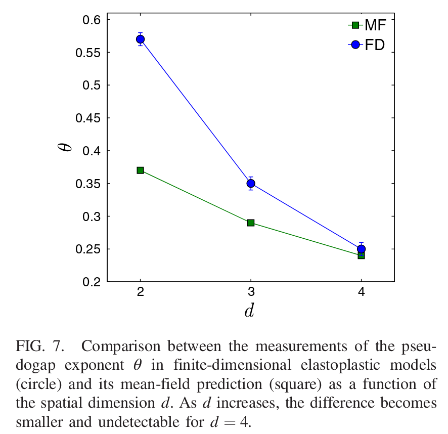
Perhaps the most interesting open question from the problem is the role of spatial dimension. One thing Lin and Wyart oobserve is that their mean field predictions get better as the dimension increases, which they mark as evidence that their mean field model is correct.

To get this behaviour they need to somehow extract \(\theta\) for finite dimensional systems. They do this by simulating according to Eq \ref{eqn:model} with a shuffled Eshelby kernel. To determine \(\theta\), they simulate the system with the kernel undergoing a random reshuffling after each event, and measure \(P(x)\) nclose to 0. To comput predictions they need the ratio \(A/v\) which ends up being equivalent to determining \(A_0\), the amplitude of the power law distrobution of the Eshelby kernel (which you can derive by looking at the max value of \(\mathcal{P}(\mathcal{G})\)).
Possible calculation routes to follow.